Determinations of the Slope of the Chao Phraya Riverbank
and Manning's Roughness Coefficient Utilizing Precise Point
Positioning (PPP) Measurement Technique
Thammaboribal, P.,1* Tripathi, N. K.,1
Nakamura, S.2 and Lipiloet, S.3
1Asian Institute of Technology, School of Engineering and
Technology, P.O. Box 4, Klong Luang, Pathumthani 12120, Thailand.
2International Relations and Research Department Japan
Aerospace Exploration Agency (JAXA), Japan
3Department of Civil Engineering, Faculty of Engineering,
Rajamangala University of Technology Thanyaburi, Pathumthani 12120, Thailand
E-mail: prapasgnss@gmail.com*
ORCID ID: 0000-0001-5885-148X
*Corresponding Author
Abstract
Flooding in Thailand, particularly in the Chao Phraya River basin,
is a recurrent challenge exacerbated by seasonal monsoons. The
catastrophic 2011 floods highlighted the urgent need for accurate
flood prediction and management strategies. This study aimed to
enhance flood modeling through precise determination of riverbank
slopes and Manning's roughness coefficients using Global Navigation
Satellite Systems (GNSS) and Precise Point Positioning (PPP)
techniques. Elevation data were collected along the riverbanks from
Ayutthaya to Bangkok using various GNSS positioning methods, with
CSRS-PPP identified as the most reliable technique for height
difference measurements. The study determined the river's slope to
be approximately 0.00003, translating to a gradient of 1:33,333.
Manning's roughness coefficients were calculated using observed
discharge data and were found to range between 0.035 and 0.045
across different river stations. The derived roughness coefficients
were validated against actual discharge measurements, revealing
seasonal variations in flow resistance. The study further
established empirical relationships between river depth,
cross-sectional area, hydraulic radius, and discharge, enabling more
accurate hydrological modeling. The results contribute to improved
flood prediction and mitigation strategies by offering a reliable
methodology for terrain elevation assessment and flow rate
estimation in flood-prone regions.
Keywords: Chao Phraya river, Discharge, Flow velocity,
GNSS, PPP, Slope
1. Introduction
Flooding is a recurring disaster in Thailand, frequently exacerbated by
the seasonal southwest monsoon, which occurs between May and November.
This rainy season leads to significant flood events, often causing
extensive damage throughout the country. In 2011, Thailand experienced
an extraordinary event referred to as the “mega flood,” which affected
65 out of the 77 provinces [1]. The flooding began in late October,
persisted through the central and northern regions, and continued into
January 2012, primarily impacting the Chao Phraya River basin [2].
The 2011 flooding caused widespread devastation, with over 800 deaths
and more than 13.6 million people affected [3]. The industrial sector
was severely impacted, particularly in large industrial estates that
had never previously experienced flooding. This event revealed a
critical gap in flood management: the lack of timely and accurate flood
data, including flow rates, runoff volumes, and water depths [4]. As a
result, people were ill-prepared to protect their properties, and the
damage was far more extensive than expected. This highlights the
crucial role that reliable flood information plays in disaster
preparedness and mitigation planning [5]. The 2011 flood serves as a
stark reminder of the need for advanced tools and methodologies to
predict flooding events and mitigate their impacts. Accurate flood
modeling, informed by up-to-date data on topography, flow rates, and
terrain characteristics, is essential to improving flood response
strategies and enhancing resilience in flood-prone regions [6][7] and
[8].
Flood dynamics are influenced by several factors, with water flow rates
primarily determined by the slope of the terrain and the roughness of
the water channel [9] and [10]. Traditionally, slope calculations rely
on differential leveling techniques, which involve the use of leveling
instruments like the “level and rod”. While effective, this method is
time-consuming and expensive [11], particularly for large regions such
as the Chao Phraya River basin in central Thailand.
Recent advancements in Global Navigation Satellite Systems (GNSS) have
provided an alternative method for determining terrain elevation
[12][13] and [14]. GNSS-derived “ellipsoid heights” can be converted
into orthometric heights through Earth gravitational models (EGM),
allowing for efficient topographic mapping of large areas [11]. Once
terrain heights are established, the slope of the area can be
calculated. Additionally, the water discharge can be modeled using
Manning's equation, which considers the slope and cross-sectional area
of the water flow, enabling the prediction of water travel time to
specific areas [15] and [16]. This study aims to enhance flood modeling
capabilities for the Chao Phraya River basin through the following
objectives: (1) To measure the terrain elevation along the riverbanks
from Ayutthaya to Bangkok using various GNSS techniques (single
positioning, static positioning, and Precise Point Positioning (PPP))
and determine the optimal technique for data collection. (2) To compute
the slope of the Chao Phraya River basin. (3) To back-calculate
Manning's roughness coefficient (n-value) from cross-sectional
parameters and the slope of the terrain. (4) To compute the flow rate
of the Chao Phraya River using Manning's equation for open channel
flow. And (5) to compare the computed discharge values with observed
data from the Royal Irrigation Department of Thailand.
By achieving these objectives, the study seeks to improve flood
prediction and management in the Chao Phraya River basin, contributing
to better preparedness for future flood events.
2. Theoretical Backgrounds
2.1 Study Area
The Chao Phraya River is a significant watercourse in Thailand, flowing
entirely within the country and covering an approximate area of 160,000
km2 [17]. The river traverses the central region of Thailand, which is
characterized by a low alluvial plain. The Chao Phraya River originates
at the confluence of the Ping and Nan rivers in Pak Nam Pho, located in
Nakhon Sawan province [18], as illustrated in Figure 1. From this
point, the river flows southward for 375 kilometers [19], passing
through the central plain of Bangkok, the capital of Thailand, before
draining into the Gulf of Thailand, which is part of both the Pacific
Ocean and the South China Sea.
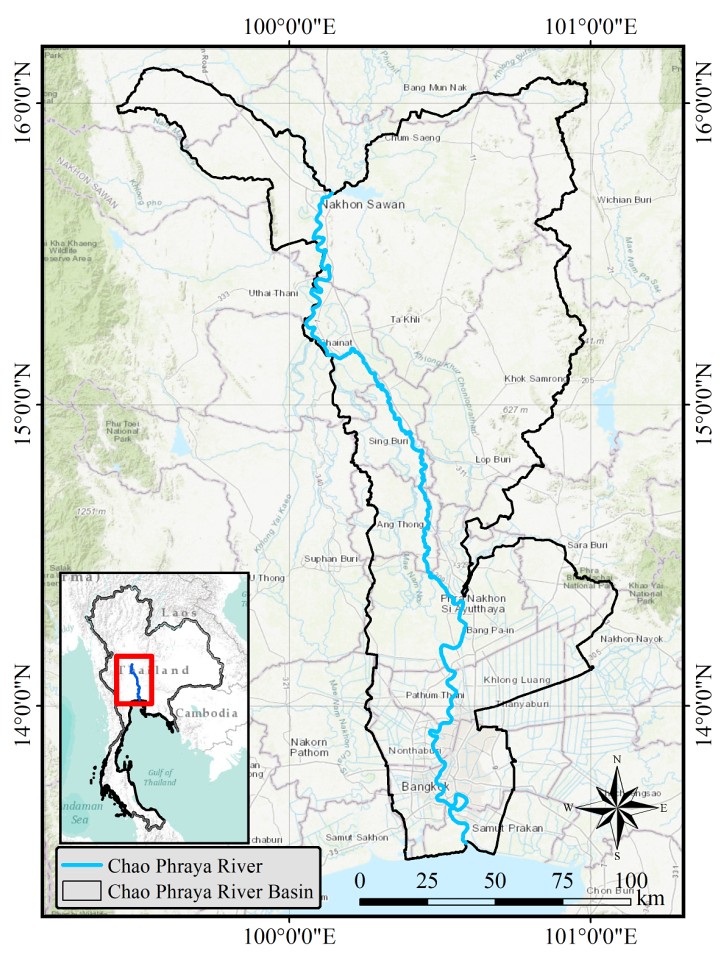
Figure 1: The Chao Phraya River, Basin
The river's approximate geographic coordinates are 13.58°N-15.67°N,
100.10°E -101.00°E [20]. The region experiences a wet monsoon climate,
with annual rainfall exceeding 1,400 millimeters [21]. The rainy season
lasts from May to October, supplemented by occasional storm depressions
originating in the Pacific Ocean. The annual average temperatures in
the area is approximately 27°C, with the maximum, temperature of 40°C
in April [22], except in higher altitude regions. The basin itself is
classified as a tropical rainforest, supporting a high level of
biodiversity. The landscape surrounding the Chao Phraya River is a
flat, expansive, and well-watered plain that is continuously replenished
with soil and sediment carried by the river. In the northern part of
the river basin, elevations exceed 20 meters, while the lower reaches
of the river feature flat terrain, with an average elevation of
approximately 2 meters above mean sea level. The region is composed of
alluvial plains that support highly productive agricultural activities.
Annual precipitation within the Chao Phraya River basin ranges from a
minimum of 1,000 mm in the western regions to about 1,400 mm in the
headwaters and up to 2,000 mm in the eastern Chao Phraya delta [23].
These precipitation values vary annually, contributing to both droughts
and floods. Approximately 85% of the annual runoff occurs between July
and December, with relatively low natural flows from January to June.
The average annual discharge of the river is approximately 883 cubic
meters per second (cms) [24]. The hydrological cycle of the Chao Phraya
River begins in April, when discharge levels typically reach their
minimum. From May to August, discharge gradually increases, with a more
rapid rise observed between August and October. Discharge levels then
decrease quickly in November and December, before slowing again until
the next minimum flow period in April. During the January to April
period, discharge typically ranges from 50 to 200 cms. The depth of the
river varies between 5 and 20 meters, while its width spans from 200 to
1,200 meters [20].
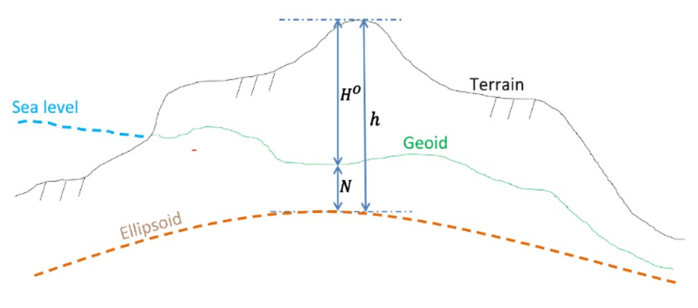
Figure 2: Ellipsoid height and orthometric height [25]
2.2 Ellipsoid Height
Ellipsoid height is defined as the vertical distance above the
reference ellipsoid, which is a mathematical model used to approximate
the Earth's shape. In contrast, orthometric height refers to the
vertical distance above the geoid, an imaginary surface that
approximates mean sea level (MSL) and is influenced by Earth's gravity
field (Figure 2). The relationship between ellipsoid height
(h) and orthometric height (H0) can be
expressed by Equation 1.
h ≈ H0 + N
Equation 1
The ellipsoid height (h) refers to the elevation above the
reference ellipsoid, which serves as an approximation of the Earth's
surface, whereas orthometric height is measured relative to an
imaginary surface called the geoid. The geoid, determined by the
Earth's gravitational field, is commonly approximated by the mean sea
level (MSL). The signed difference between the ellipsoid and geoid
surfaces is known as the geoid undulation (N), which arises
because the direction of the plumb line (the normal to the geoid)
differs from the normal to the ellipsoid [25]. Geoid undulation values
are computed by applying corrected values that convert pseudo-height
anomalies, calculated at a point on the ellipsoid, into corresponding
geoid undulation values [26]. The Earth Gravitational Model (EGM),
developed and published by the National Geospatial-Intelligence Agency
(NGA), is commonly employed for determining geoid undulation. The
Office of Geomatics at NGA is responsible for the collection,
processing, and evaluation of gravity data, including free-air and
Bouguer gravity anomalies [27]. Gravimetric quantities such as mean
gravity anomalies, geoid heights, and gravity disturbances are derived
from the collected data. The EGM models published by NGA include EGM84,
EGM96, and EGM2008, with the most recent version, EGM2008, being
publicly available. EGM2008 is defined up to spherical harmonic degree
and order 2159, with additional coefficients extending to degree 2190
and order 2159 [28]. Model coefficients can be accessed online at
https://earth-info.nga.mil/. Geoid height can be computed online via
the tool at
https://earth-info.nga.mil/index.php?dir=wgs84&action=egm96-geoid-calc,
and
https://geographiclib.sourceforge.io/cgi-bin/GeoidEval where users
input the receiver's position to automatically calculate the geoid
heights for various EGM models.
2.3 Precise Point Positioning
GNSS receivers operating in favorable weather conditions with good
satellite availability can achieve coordinates with horizontal accuracy
of approximately 3–5 meters and vertical accuracy of 6–10 meters,
within a 95% confidence interval [29][30] and [31]. The main sources of
error in GNSS coordinates include atmospheric delays (ionospheric and
tropospheric), satellite clock corrections, satellite geometry, and
site-dependent effects such as multipath interference and measurement
noise [32][33] and [34]. Physical obstructions that weaken satellite
geometry can block satellite signals, resulting in degraded position
accuracy [35].
Precise Point Positioning (PPP) is a technique that models or removes
errors in the GNSS system to achieve high positioning accuracy using
only a single GNSS receiver[36]. PPP accuracy primarily depends on
corrections to satellite orbits and satellite clocks. This method can
achieve decimeter-level positioning or better without requiring a base
station [37]. The PPP solution requires a convergence period to
achieve decimeter-level accuracy, allowing the resolution of local
biases such as multipath effects, satellite geometry, and atmospheric
conditions. The convergence time is influenced by the quality of the
corrections and their application in the receiver. Under optimal
conditions, PPP can achieve accuracy levels as precise as three
centimeters [11]. When processing IGS orbits, Earth orientation
parameters, and satellite clock corrections, various products are
freely available at:
https://cddis.nasa.gov/Data_and_Derived_Products/GNSS/orbit_and_clock_products.html.
.4 Manning's Roughness Coefficient
The roughness coefficient in open channel flow is a numerical value
that quantifies the resistance to flow caused by the roughness of the
channel bed and sides. It is used in hydraulic engineering to estimate
frictional losses in flowing water and is a key parameter in Manning's
equation, which is commonly applied to calculate flow velocity and
discharge in open channels, as shown in Equation 2 [38].
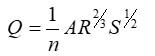
Equation 2
Where: Q is discharge, n is Manning's roughness
coefficient, A is cross-sectional area of flow, Ris
hydraulic radius (ratio of the cross-sectional area to the wetted
perimeter), and S is slope of the flow. The typical values of
n presents in Table 1.
3. Methodology
This study is divided into three main parts. The first part focuses on
assessing the performance of height measurements using a GNSS receiver,
comparing the heights derived from conventional leveling and GNSS
methods. The second part involves determining the slope of the Chao
Phraya River basin by collecting elevation data along the riverbanks,
from Ayutthaya to Bangkok province. The third part addresses the flow
rate (or discharge) of the Chao Phraya River, using Manning's method to
back-calculate the Manning's roughness coefficient. The river velocity
will be determined once the discharge is known. Finally, the computed
discharge will be compared with actual discharge data collected by the
Royal Irrigation Department of Thailand. The study workflow illustrates
in Figure 3.
3.1 Study Workflow
According to Figure 3, the reliability of the heights derived from a
GNSS receiver was assessed by setting up seven stations in the
mountainous area of Lamphrayaklang Sub-district, Muaklek District,
Saraburi Province. The height at each station was determined using the
differential leveling method with levels and rods, and was also
measured using a GNSS receiver at the same points. The GNSS heights were
determined using various techniques, including single positioning, PPP
via RTKLib, online PPP, and DGPS by RTKLib. The ellipsoidal heights
derived from the GNSS receiver were converted to orthometric heights
using the EGM08 model. The height differences calculated from both
measurement methods were then compared to evaluate the performance and
reliability of orthometric height determination using the GNSS
receiver. The slope of the Chao Phraya River basin was determined by
placing the GNSS receiver along the riverbank, from Ayutthaya Province
to Bangkok. Data were collected at each station for one hour and stored
as RINEX files. The coordinates and ellipsoidal heights of each station
were determined using several techniques: single positioning, static
positioning (rnx2rtkp), RTKLib PPP, and online PPP.
Table 1: Manning's roughness coefficient [39]
|
Class
|
Description
|
Minimum
|
Normal
|
Maximum
|
|
a
|
Clean, straight, full stage, no rifts or deep
pools
|
0.025
|
0.030
|
0.033
|
|
b
|
Same as above, but more stone and weeds
|
0.030
|
0.035
|
0.040
|
|
c
|
Clean, winding, some pools and shoals
|
0.033
|
0.040
|
0.045
|
|
d
|
Same as above, but some weed and stone
|
0.035
|
0.045
|
0.050
|
|
e
|
Same as above, lower stages, more ineffective
slopes and sections
|
0.040
|
0.048
|
0.055
|
|
f
|
Same as “d” with more stone
|
0.045
|
0.050
|
0.060
|
|
g
|
Sluggish reaches, weedy, deep pools
|
0.050
|
0.070
|
0.080
|
|
h
|
Very weedy reaches, deep pools, or floodways with
heavy stand of timber and underbrush
|
0.075
|
0.100
|
0.150
|
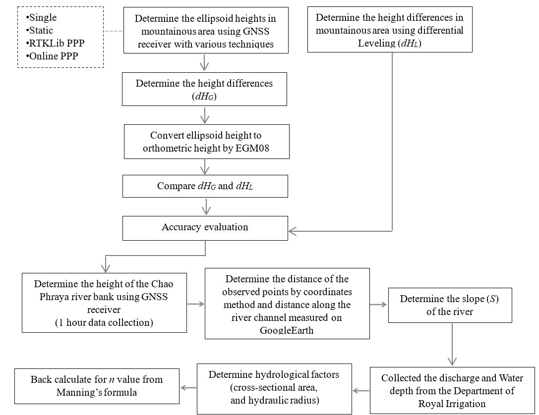
Figure 3: The slope of the Chaophraya River and
manning coefficient determination workflow
The ellipsoidal heights were then converted to orthometric heights
using geoid undulations obtained from the EGM08 geoid model. Finally,
the slope of the study area was determined by calculating the
relationship between the distances and height differences of the
collected points. Manning's roughness coefficient for the river was
back-calculated using Manning's formula. The computed discharge was
then compared with the real discharge observed by the Department of
Royal Irrigation.
3.2 Data collection
Data was collected using a “Javad” Sigma GNSS receiver as shown in
Figure 4. Each observation station recorded satellite signals for one
hour. The stations were located along the Chao Phraya River, from
Ayutthaya Province to Bangkok. The collected data were converted into
RINEX files using "Netview" software, with a data collection rate of 1
Hz. These RINEX files were then used to compute the coordinates and
ellipsoidal heights of the observed stations. A tripod was not required
for instrument setup, as the receiver is placed directly on the ground
surface. Since the receiver heights are uniform, the terrain height
will not be affected by the receiver height, meaning the height of the
receiver can be neglected in the height difference calculations. Twelve
observation stations were selected in areas that can be accessed without
special permission, such as temples and schools. The locations of the
observed stations along the Chao Phraya River bank are shown in Figure
5.
3.3 Post Processing
The RINEX files were used in the post-processing phase to determine the
coordinates and ellipsoidal heights of the observed stations. Various
techniques were employed to compute the receiver positions and
ellipsoidal heights.
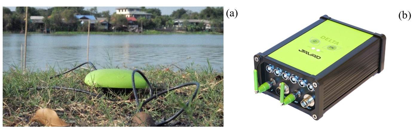
Figure 4: GNSS measurement (a) field data collection
(b) Javad Sigma GNSS receiver
Table 2: RTKLib static positioning parameter
descriptions [40]
|
Parameters
|
Description
|
|
-p
|
0:single, 1:dgps, 2:kinematic, 3:static,
4:moving-base, 5:fixed, 6:ppp-kinematic,
7:ppp-static)
|
|
-f
|
number of frequencies for relative mode
(1:L1,2:L1+L2,3:L1+L2+L5)
|
|
-t
|
output time in the form of yyyy/mm/dd hh:mm:ss.ss
[sssss.ss]
|
|
-e
|
output x/y/z-ecef position
[latitude/longitude/height]
|
|
-s
|
field separator [' ']
|
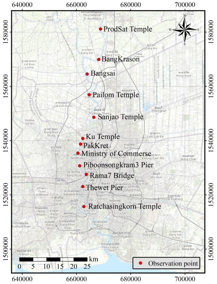
Figure 5: Data collection points for slope measurement
along the Chao Phraya River
3.3.1 Static positioning by RTKLib
The RINEX observation file contained the observations data from the
field (rover). In relative mode, the second RINEX observation file
contained the observation from the reference (base station) receiver.
The base file is downloaded from the Chulalongkorn station (CUSV)
reference station, available at:
https://cddis.nasa.gov/archive/gnss/data/daily/. Post-processing using
the static positioning technique was initiated with the command
>rnx2rtkp -p 3 -f 2 -t -e -s, RINEX_observation_file.o
Base_station_file.o_station Navigation_file.n >Outp ut_file.txt
. The detail of the code above shown in Table 2. The coordinates
obtained from rnx2rtkp are in the ECEF reference frame, so they must be
converted to geographic coordinates.
3.3.2 Precise Point Positioning
3.3.2.1 RTKLib
Precise Point Positioning (PPP) can be performed using RTKLib with
orbit (.sp3)and clock products (.clk) from the IGS. Unlike traditional
high-accuracy positioning techniques, PPP does not require a base
station to be set up. Instead, it utilizes highly accurate clock and
orbit products derived from a global network of reference stations.
This allows users to achieve centimeter-level accuracy without being
limited by the distance from any particular base station. The orbit and
clock products are available on the IGS website and are derived from a
global network of continuously operating reference stations maintained
by both public and private organizations. RTKPOST in RTKLib software is
one of several PPP tools that users can access free of charge [40].
3.3.2.2 Online precise point positioning using the Natural
Resources Canada Canadian Spatial Reference System (CSRS-PPP)
Precise Point Positioning (PPP) is a GNSS data processing technique
that can generate highly precise coordinates. The algorithm behind this
technique is somewhat complex, so using online PPP services is a
convenient way to obtain more accurate coordinates. For this study, the
Canadian Spatial Reference System PPP service (CSRS-PPP) was used to
determine the coordinates and ellipsoidal heights of the points in the
study area. The CSRS-PPP service is available online at
https://webapp.csrs-scrs.nrcan-rncan.gc.ca/geod/tools-outils/ppp.php?locale=en.
Generally, more accurate coordinates and ellipsoidal heights can be
obtained with longer data files, with 24-hour files being preferable
[41] and [42]. However, shorter files can still provide sufficient
accuracy, especially when precise satellite orbit and clock data are
available.
3.3.2.3 Online precise point positioning using the GNSS analysis
and positioning software (GAPS-PPP)
Online PPP can also be performed via the website
http://gaps.gge.unb.ca/submitbasic.php, which is provided by the
University of New Brunswick, Canada [43]. RINEX observation files are
submitted through the website for processing, and the results are sent
back to the user's specified email.
One advantage of this service over CSRS-PPP is that the coordinates of
the observed points can be visualized in Google Earth using a .kml
file. Additionally, the overall results can be accessed on any web
browser.
3.4 Discharge Data Acquisition
The flow data and cross-sectional data were downloaded from the Office
of Water Management and the Hydrology Department of the Royal
Irrigation Department of Thailand at
http://hydro-5.rid.go.th/. The
data were collected from in November 2024. In this study, observation
stations C35, C36, and C37 were selected because they are located in
Phranakhon Si Ayutthaya Province (Figure 6), where the study area
begins, and the river slope data collection started in this region. The
cross-sections and water depths of the three observation stations are
depicted in Figure 7.
4. Results and Discussion
4.1 Differential Leveling and GNSS Heights
Height differences were measured using both differential leveling and
GNSS techniques, and the results from both methods were compared. Three
observation points with known coordinates and elevations were
established. The GNSS receiver was then placed at each point to
determine the elevation. The results are presented in Figure 8 and Table
3. The table shows that single point positioning is not suitable for
height determination, as the accuracy varies from 4 to 6 meters. The
orthometric heights derived from GNSS, computed using Precise Point
Positioning (PPP) with both CSRS and GAPS, as well as the Static
Positioning (rnx2rtkp) technique, are quite similar to each other. The
elevations of the terrain derived from both GNSS techniques are
approximately one meter lower than the true orthometric heights. This
discrepancy is due to the fact that the orthometric heights in the study
area are based on the local geoid at Koh Lak, Prachuapkirikhan
Province, Thailand, whereas the GNSS-derived orthometric heights are
based on the global geoid (ITRF). Therefore, orthometric heights
derived from GNSS receivers are not suitable for determining terrain
elevations.
Table 3: Differences in orthometric heights between
conventional leveling and PPP
|
Station No.
|
Errors = Fixed – Measurement Techniques [m]
|
|
Single
Pos.
|
Static (Rnx2rtkp)
|
CSRS
PPP
|
GAPS
PPP
|
RTKLiB
PPP
|
|
1
|
-6.251
|
-0.808
|
-0.940
|
-0.981
|
-1.642
|
|
2
|
-4.422
|
-0.989
|
-1.222
|
-1.250
|
-0.904
|
|
3
|
4.979
|
-0.978
|
-1.011
|
-0.756
|
-0.804
|
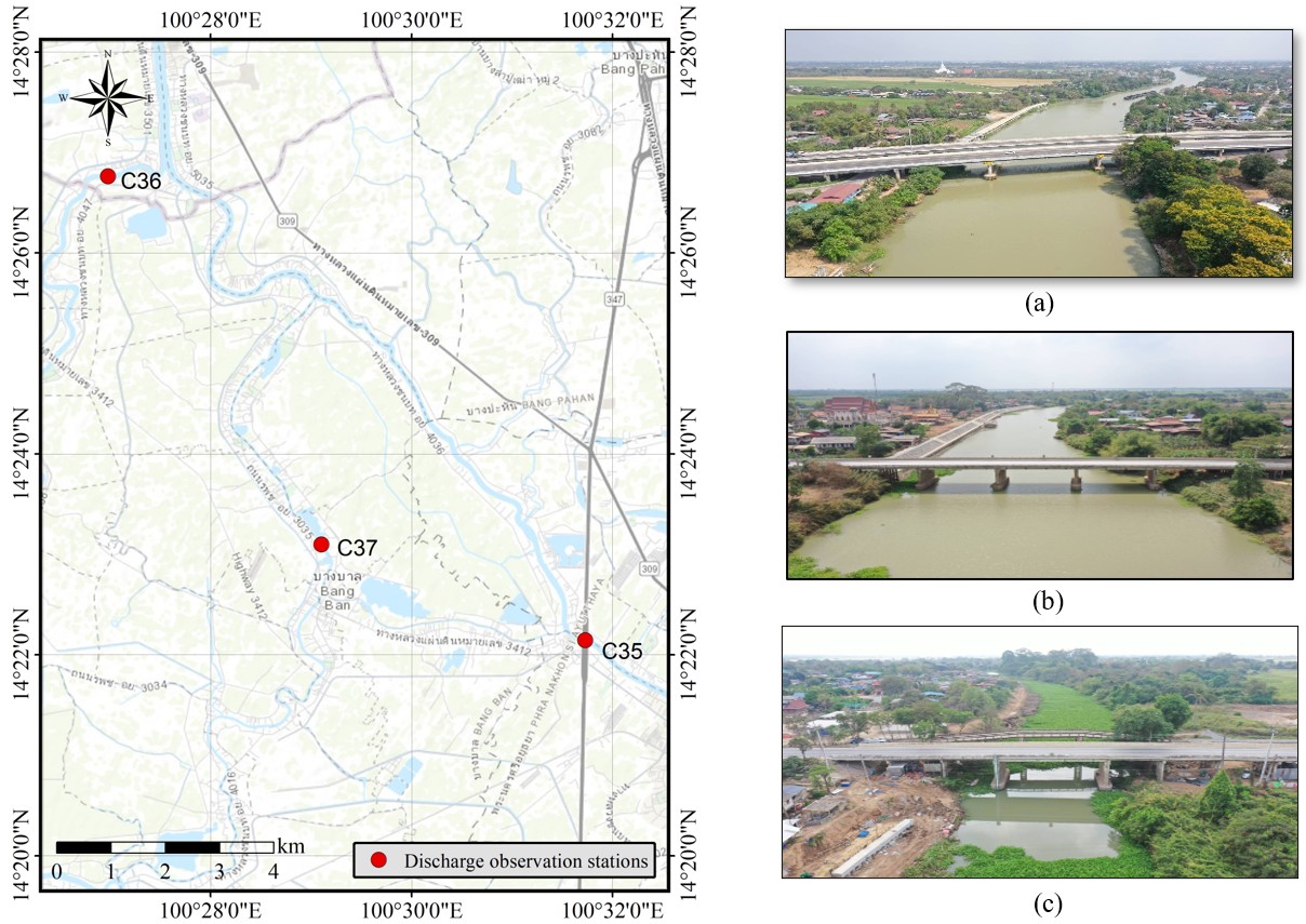
Figure 6: Observation stations (a) C35 (b) C36 (c) C37
in Phranakhon Si Ayutthaya province
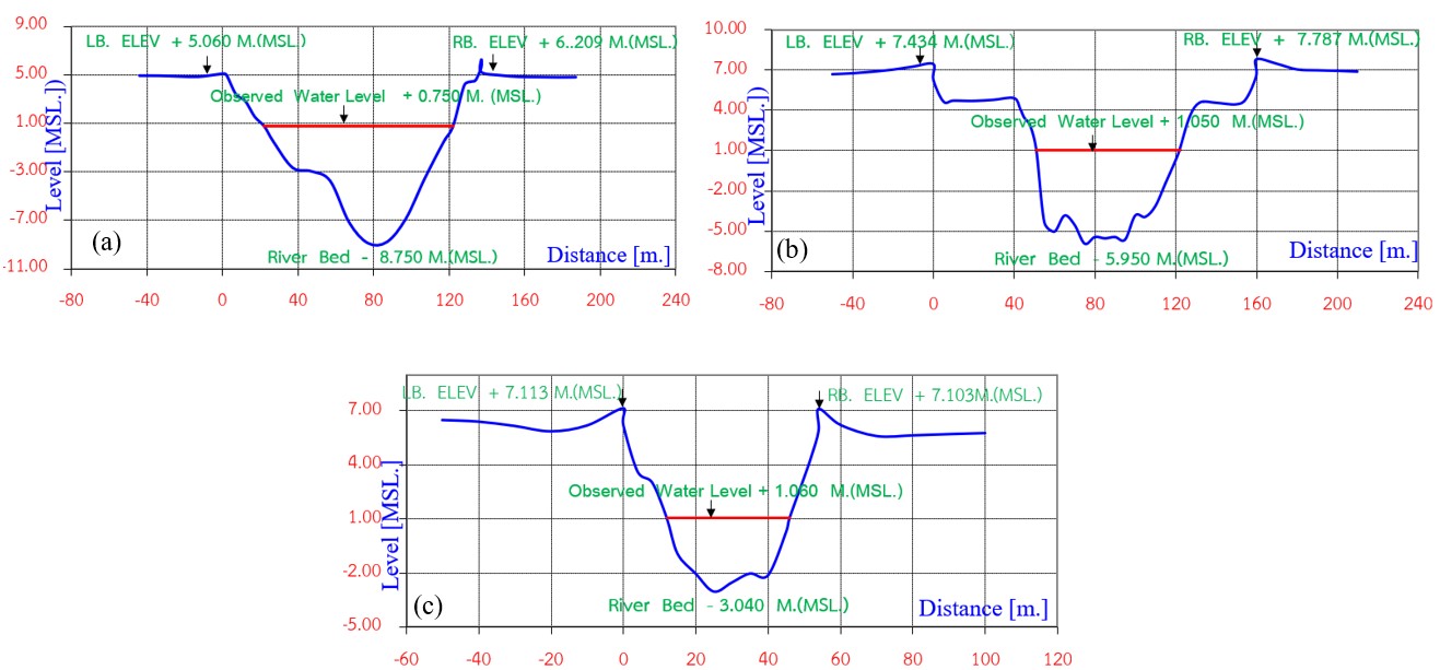
Figure 7: Cross-sections of the river at the
observation stations (a) C35 (b) C36 (c) C37
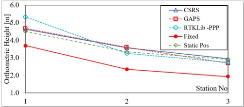
Figure 8: Comparison of orthometric heights obtained
from conventional leveling and PPP
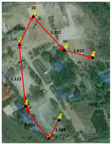
Figure 9: Differential leveling test site
4.2 Assessment of Orthometric Height Derived from Ellipsoid Height
Based on the previous section, it is clear that the elevations derived
from the GNSS receiver are approximately one meter above the actual
terrain, raising questions about the feasibility of using GNSS
elevation data to determine terrain heights. However, GNSS receivers
may still be useful for measuring height differences, making it crucial
to validate the height differences derived from GNSS data. Validation
was conducted in the mountainous area of Muak Lek District, Saraburi
Province, Thailand. Seven stations were established to measure height
differences using both conventional leveling and GNSS techniques. The
leveling test site and the leveling points present in Figure 9. Table 4
presents the geoid undulations and ellipsoid heights calculated using
different computation methods. The orthometric height of each station
was determined from Equation 1. The orthometric heights and height
differences present in Table 5 and Figure 10, respectively. Since
conventional leveling provides the orthometric heights of the terrain
and is commonly used to determine height differences, it serves as the
reference method for assessing the errors of height differences computed
by other techniques. Table 5 and Figure 10 demonstrate that the height
differences computed using online PPP, specifically both CSRS and GAPS,
are in close agreement with the results from differential leveling.
Table 4: Geoid undulation and ellipsoid heights
|
Station No.
|
Geoid undulation
[m]
|
Ellipsoid height [m]
|
|
CSRS
PPP
|
GAPS
PPP
|
RTKLib
PPP
|
Static
Pos.
|
Single
Pos.
|
|
1
|
-29.694
|
215.715
|
215.723
|
215.596
|
215.076
|
216.513
|
|
2
|
-29.693
|
216.970
|
217.163
|
217.379
|
216.624
|
223.120
|
|
3
|
-29.695
|
217.586
|
217.890
|
217.189
|
217.757
|
217.211
|
|
4
|
-29.698
|
216.384
|
216.241
|
215.935
|
217.861
|
213.365
|
|
5
|
-29.699
|
215.315
|
215.335
|
215.184
|
215.300
|
215.766
|
|
6
|
-29.697
|
219.126
|
219.135
|
218.513
|
219.003
|
218.178
|
|
7
|
-29.696
|
220.958
|
220.894
|
220.807
|
221.110
|
218.606
|
Table 5: Orthometric heights derived from ellipsoid
heights and geoid undulations
|
Station No.
|
Orthometric height [m]
|
|
CSRS
PPP
|
GAPS
PPP
|
RTKLib
PPP
|
Static
Pos.
|
Single
Pos.
|
|
1
|
186.022
|
186.029
|
185.902
|
185.383
|
186.820
|
|
2
|
187.277
|
187.470
|
187.686
|
186.931
|
193.427
|
|
3
|
187.891
|
188.195
|
187.494
|
188.062
|
187.516
|
|
4
|
186.686
|
186.543
|
186.237
|
188.163
|
183.667
|
|
5
|
185.616
|
185.636
|
185.485
|
185.601
|
186.067
|
|
6
|
189.429
|
189.439
|
188.817
|
189.306
|
188.481
|
|
7
|
191.263
|
191.199
|
191.112
|
191.415
|
188.911
|
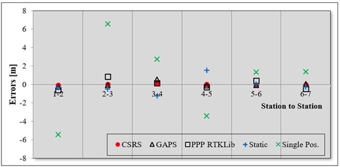
Figure 10: Error of height differences between
differential leveling and GNSS measurement
The height differences between the points in the test area calculated
by the online PPP methods are nearly identical to those derived from
differential leveling, whereas other computation techniques exhibit
higher errors and more significant deviations from the leveling
results. Therefore, height differences derived from the GNSS receiver
using online PPP provide the best match with differential leveling
data. Figure 10 further illustrates that CSRS-PPP produces height
differences that are closer to those obtained from differential
leveling compared to GAPS-PPP. As shown in the figure, the red circle is
positioned near the zero error line, which represents the differential
leveling result. This suggests that orthometric heights can be
accurately computed from the ellipsoid height derived from CSRS-PPP,
indicating that GNSS receivers are highly suitable for determining
height differences.
Furthermore, Figure 10 clearly shows that the CSRS-PPP technique yields
the smallest error in height differences, followed by GAPS-PPP, RTKLib
PPP, static (rnx2rtkp), and single positioning, in that order. The
error range for height differences computed using CSRS-PPP is between
0.01 and 0.08 meters, while GAPS-PPP shows errors between 0.05 and 0.50
meters.
Based on these results, the CSRS-PPP technique was selected for
determining the height of the Chao Phraya River bank to investigate the
slope of the river basin. In conclusion, the results of the height
difference determinations suggest that GNSS receivers are capable of
accurately determining height differences, especially in areas where
observation points are widely spaced. The "Online Precise Positioning
Point (PPP)" computation method provides the closest approximation of
height differences when compared to the conventional leveling
technique.
4.3 Slope of the Chao Phraya River Basin
Since the online PPP technique provides the most accurate height
difference values compared to conventional leveling, the GNSS receiver
was employed to determine the terrain heights along the Chao Phraya
River for slope analysis in the study area. The measurements were
conducted from Ayutthaya Province to Pathum Thani, Nonthaburi, and
Bangkok. A total of twelve observation stations were established along
the river, with data collected using a Javad GNSS receiver. Each
station collected data for approximately one hour, and post-processing
was performed using the CSRS-PPP tool at
https://webapp.csrs-scrs.nrcan-rncan.gc.ca/geod/tools-outils/ppp.php?locale=en.
The distances between the observation points were measured along the
river using Google Earth.
Figure 11 illustrates that the slope of the Chao Phraya River is
relatively flat, with a slope of 0.00003, approximately corresponding
to 1:33,333. The coefficient of determination (r2) is approximately
0.82, indicating that 82% of the variation in elevation can be
explained by the distance between observation points. The result is in
perfect alignment with the previous study [44]. These results suggest
that the Chao Phraya River basin exhibits a north-to-south gradient.
Additionally, the results validate the slope measurements obtained using
a GNSS receiver, as the river flows from the northern region toward the
Gulf of Thailand in the south. The elevation at Nakhon Sawan Province
is approximately +20 meters above mean sea level (MSL), while Bangkok's
elevation is approximately +2 meters MSL. The distance between these
two provinces is approximately 375 kilometers. Based on this data, the
approximate slope of the Chao Phraya River basin is 0.000048. However,
since the measurement does not follow the river's exact course, some
measurement error may be present. Despite this, a slope ratio of
1:33,333 is considered sufficiently accurate for use in hydrological
modeling.
4.4 Manning's Roughness Coefficient Estimation
The slope of the study area was determined in the previous section, and
the Manning coefficients for the Chao Phraya River were calculated
using Manning's formula (Equation 2). Data for discharge computations
were sourced from the Department of Royal Irrigation of Thailand,
available at:
http://hydro-5.rid.go.th/. Discharge, cross-sectional
area, and river width data were collected and utilized in the
back-calculation of Manning's coefficients. Several monitoring stations
along the Chao Phraya River begin in Nakhon Sawan Province (station
C2), but only three stations in Ayutthaya Province (C35, C36, and C37),
as shown in Figure 6, were considered for this analysis. These
stations were selected due to the availability of slope measurements
and river cross-sectional data in this region.
Manning's formula, presented in Equation 2, allows for the calculation
of discharge in an open channel. Given known values for discharge,
width, and cross-sectional area of the river, the Manning roughness
coefficient can be determined. The Manning coefficients were
back-calculated from the data provided in Table 6.
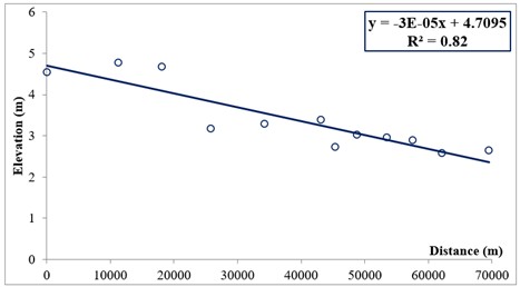
Figure 11: Determination of the slope of the Chao
Phraya River
Table 6: The back-calculation of Manning's roughness
coefficients
|
Station
|
C35
|
C36
|
C37
|
|
Cross sectional area; A (sq.m)
|
516.445
|
252.43
|
102.5
|
|
Wet perimeter; P (m)
|
107.09
|
75.13
|
35.24
|
|
Hydraulic radius; R (m)
|
4.82
|
3.36
|
2.91
|
|
Discharge; Q (cms)
|
228
|
80.54
|
25.48
|
|
Slope; S
|
1:33333
|
|
Manning's roughness coefficients; n
|
0.035
|
0.039
|
0.045
|
Table 7: Hydrological parameters for discharge and
flow velocity
|
Station
|
Cross sectional area; A [sq.m.]
|
Hydraulic radius;
R [m.]
|
Discharge
[cms]
|
Velocity
[m/s]
|
|
C35
|
A=128.64 y + 361.71
|
R=4.5895 y + 0.4182
|
Q=19.521 y2 + 192.61
y + 47.507
|
V=0.233 y + 0.355
|
|
C36
|
A=76.701 y + 259.96
|
R=4.1499 y + 1.604
|
Q=6.122 y2 + 67.342
y + 37.94
|
V=0.160 y + 0.136
|
|
C37
|
A=37.976 y + 74.954
|
R=7.4503 y + 0.7885
|
Q=3.201 y2 + 22.179
y + 4.6333
|
V=0.163 y + 0.076
|
The manning's roughness coefficients at stations C35, C36, and C37 are
0.035, 0.039, and 0.045, respectively. The average value of the
coefficient is 0.040. The manning's coefficient at each station are not
identical because of several factors that influence flow resistance.
These include the composition of the riverbed, such as the presence of
sand, gravel, or rocks; the type and density of vegetation, which can
increase roughness, and the shape and size of the channel, with
meanders and irregularities adding resistance [45] and [46].
Additionally, features like bank and bed obstructions, including
boulders or fallen trees, contribute to variations in roughness. The
coefficient is highest at station C37, likely due to the presence of
weeds and water hyacinth covering the riverbank at this location [47]
(see Figure 6(c)). The Manning's roughness coefficients derived from
this study can be informative and useful to be used in hydrogogical
model as SWAT and HEC-RAS models [48].
4.5 Verification of the Manning's Roughness Coefficient
Since the Manning's n values were derived from flow data,
their accuracy must be verified to ensure they are suitable for
discharge computations in the Chao Phraya River. Essential parameters
for discharge calculation include the cross-sectional area and the
wetted perimeter of the channel. Typically, only the water level above
mean sea level (MSL) is measured at each observation station, and the
river's irregular shape, unlike that of man-made concrete canals, makes
it challenging to directly calculate the cross-sectional area and
wetted perimeter. As a result, discharge calculations cannot be
accurately performed without these measurements.
Discharge is usually determined using a rating curve, which represents
the relationship between water level and discharge. The velocity of
water flow can be calculated by dividing the discharge by the
cross-sectional area of the channel, enabling the plotting of the
relationship between water level and river flow velocity. As per
Equation 2, the hydraulic radius can be back-calculated, given that the
Manning's roughness coefficient, river slope, and cross-sectional area
of the channel are known.
Since cross-sectional area data are typically unavailable, and only
water levels are observed, Manning's formula cannot be applied without
knowledge of the river's cross-sectional area. Therefore, it is
essential to investigate and establish the relationship between water
level and cross-sectional area. Figure 12 illustrates this
relationship, while Figure 13 shows the correlation between water level
and hydraulic radius at stations C35, C36, and C37. The hydrological
parameters required for determining cross-sectional area (A),
hydraulic radius (R), discharge (Q) and flow velocity
(V) can be derived from the river depth (y), as
detailed in Table 7.
4.6 Validation of the Models
To validate the model parameters derived in the previous sections, the
discharges of the Chao Phraya River at stations C35, C36, and C37 on
other days were computed using the correlations presented in Figures 12
and 13, along with the Manning's n and slope values determined
in Sections 4.3 and 4.4. In this case, discharges were easily
calculated directly from the established relationships, eliminating the
need for the complex formula with multiple parameters, as shown in
Equation 2. A comparison between the actual discharges, provided by the
Department of Royal Irrigation, and the modeled discharges is presented
in Figure 14. The comparison between actual and computed discharges
reveals that at station C35, the discharge differences range from 0.04
to 59.83 cubic meters per second (cms), with a mean difference of 40.67
cms.
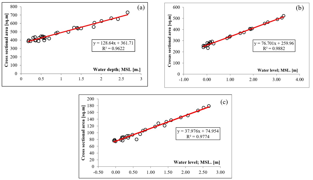
Figure 12: Correlation between river depth and cross
sectional area (a) C35 (b) C36 (c) C37
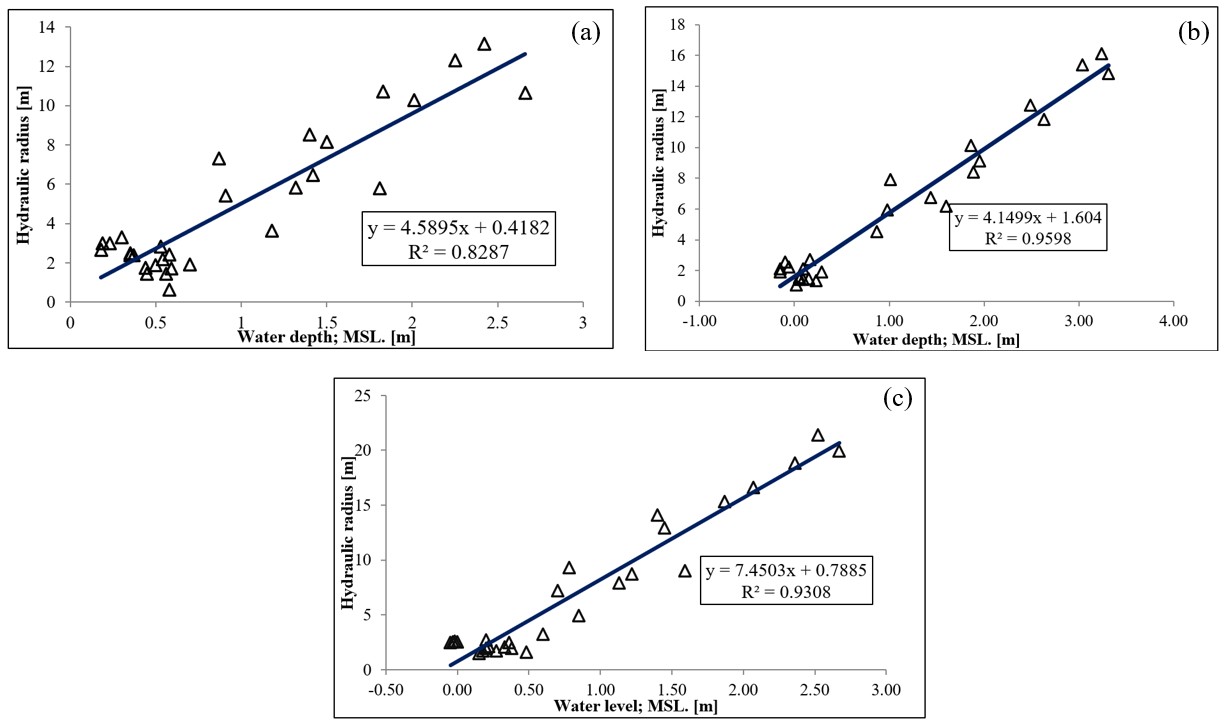
Figure 13: Correlation between river depth and
hydraulic radius (a) C35 (b) C36 (c) C37
As shown in Figure 14, the discrepancies between actual and computed
discharges are notably higher during the summer and winter seasons,
while the differences are smaller during the rainy season (August to
November). Average discharges during the summer (March to July) and
winter (November to April) are approximately 200-250 cms, whereas the
highest discharge occurs in the rainy season, with a peak of 700 cms in
August. The larger discrepancies between modeled and actual discharges
in the summer and winter can be attributed to variations in the
roughness between the water and the riverbank.
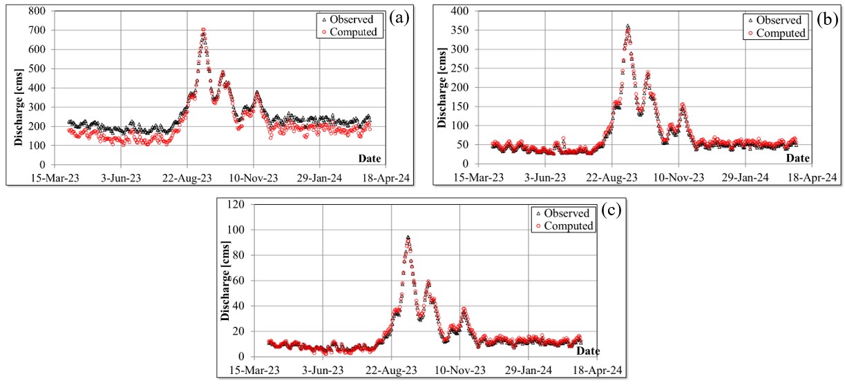
Figure 14: Comparison of actual and modeled discharge
values (a) C35 (b) C36 (c) C37
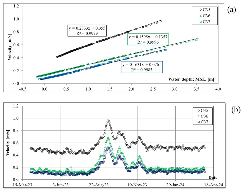
Figure 15: Velocity of river flow: (a) correlation
between river depth and velocity (b) velocity modeling
Consequently, the Manning's n values derived from the model may not
remain constant throughout the year. At station C35, the river width
is the widest compared to stations C36 and C37, which may contribute to
the higher differences observed. However, the modeled discharge aligns
well with actual discharge during the rainy season, indicating that the
derived parameters and the model are reliable for estimating discharges
during this period, which is crucial for flood assessments. At stations
C36 and C37, the comparison between computed and actual discharges
shows smaller discrepancies, with differences ranging from 0.02 to 11.76
cms at C36 and 0.03 to 3.17 cms at C37. The river widths at these
stations are smaller than at C35, and thus the Manning's n values are
less affected by variations in water depth. Therefore, the models for
stations C36 and C37 are more suitable for estimating discharge
throughout the year.
4.7 Velocity of the River Flow
The flow velocity can be easily calculated by dividing the discharge by
the river's cross-sectional area. Since the cross-sectional area is
proportional to the river depth, as depicted in Figure 12, the
velocity at each station can be estimated based on the river depth, as
shown in Figure 15. The velocities computed using Manning's formula and
those derived from the relationship in Figure 15(a) show a consistent
difference of approximately 0.01 m/s at each observed station.
This indicates that the relation in Figure 15(a) can reliably predict
river flow velocities. This is particularly valuable for determining
evacuation times during periods of high water or flooding events.
Figure 15(b) demonstrates that the velocity of the Chao Phraya River at
station C35 is approximately 0.4 m/s (34.56 km/day) during the summer
and 0.5 m/s (43.2 km/day) in winter. However, during the rainy season
(August to November), the velocity fluctuates in response to changes in
discharge. At stations C36 and C37, the velocities are similar, with
values of about 0.1 m/s (8.64 km/day) in summer and 0.2 m/s (17.28
km/day) in winter, with variations also occurring during the rainy
season. As shown in Figure 15(b), the velocity at station C35 is
approximately three times faster than at station C36 and five times
faster than at station C37.
5. Conclusions
This study successfully determined the slope of the Chao Phraya River
and Manning's roughness coefficients using GNSS-based Precise Point
Positioning (PPP) techniques. The results confirm that GNSS
measurements, particularly those processed through online PPP services
such as CSRS-PPP, provide highly accurate height differences suitable
for slope calculations. The computed slope of 0.00003 (1:33,333) aligns
with the expected topographical gradient from Nakhon Sawan to Bangkok
and previous study. Manning's roughness coefficients, essential for
flow modeling, were back-calculated using observed discharge data and
Manning's equation. The derived coefficients varied from 0.035 to
0.045, reflecting differences in riverbed characteristics, vegetation,
and channel geometry. The highest roughness coefficient was observed at
station C37, likely due to extensive vegetation along the riverbanks.
Validation of the roughness coefficients using observed discharge data
indicated that seasonal variations significantly influence flow
resistance, with higher discrepancies occurring during dry seasons due
to changes in channel morphology and sediment deposition.
Additionally, the study established empirical relationships between
river depth and hydrological parameters such as cross-sectional area,
hydraulic radius, and discharge. These relationships allow for more
efficient estimation of flow characteristics based on observed water
levels, reducing dependency on direct discharge measurements. The
velocity modeling further demonstrated the seasonal variability in river
flow rates, highlighting the importance of accurate roughness
coefficient estimation for flood forecasting. Despite the successful
implementation of GNSS-based methodologies, some limitations were
identified.
The accuracy of orthometric height conversion depends on geoid models,
and localized geoid variations may introduce minor errors. Moreover,
the study's focus on a limited number of observation stations may not
fully capture the spatial variability in riverbed conditions. Future
research should expand the dataset to include more stations and
integrate real-time monitoring techniques for continuous slope and flow
assessments.
6. Recommendation
To enhance flood prediction and management in the Chao Phraya River
basin, this study recommends integrating real-time GNSS monitoring for
improved slope and elevation data, refining geoid models for greater
accuracy, and expanding observation stations to better capture
variations in Manning's roughness coefficients. The incorporation of
remote sensing data, such as LiDAR and satellite imagery, can enhance
terrain assessments. Seasonal calibration of roughness coefficients is
necessary to account for changes in vegetation and sediment deposition.
Additionally, developing advanced predictive models that integrate
GNSS-based slope measurements and real-time discharge data will improve
flood preparedness. Public awareness and policy implementation should
also be prioritized through early warning systems and comprehensive
flood risk mapping. Implementing these strategies will strengthen
Thailand's flood resilience, minimizing the impact of future flood
events on communities and infrastructure.
References
[1] Gale, L., E. and Saunders, A., M., (2013). The 2011 Thailand
Flood: Climate Causes and Return Periods. Weather, Vol. 68(9).
223-237.
https://doi.org/10.1002/wea.2133.
[2] NASA Earth Observatory, (2011). Flooding in Thailand.
[Online]. Available:
https://earthobservatory.nasa.gov/images/76683/flooding-in-thailand.
[Accessed: Nov. 19, 2024].
[3] Promchote, P., Simon Wang, Y. S. and Johnson, G. P., (2016).
The 2011 Great Flood in Thailand: Climate Diagnostics and Implications
from Climate Change. Journal of Climate, Vol. 29(1), 367-379.
https://doi.org/10.1175/JCLID-15-0310.1.
[4] Marks, D., (2019). Assembling the 2011 Thailand Floods:
Protecting Farmers and Inundating High-Value Industrial Estates in A
Fragmented Hydro-Social Territory. Political Geography, Vol.
68, 66-76.
https://doi.org/10.1016/j.polgeo.2018.10.002.
[5] Loc, H. H., Emadzadeh, A., Park, E., Nontikansak, P. and Deo,
R. C., (5023). The Great 2011 Thailand Flood Disaster Revisited: Could
It Have Been Mitigated by Different Dam Operations Based on Better
Weather Forecasts?. Environmental Research, Vol. 216.
https://doi.org/10.1016/j.envres.2022.114493.
[6] Khunwishit, S., Choosuk, C. and Webb, G., (2018). Flood
Resilience Building in Thailand: Assessing Progress and the Effect of
Leadership. International Journal of Disaster Risk Science,
Vol. 9, 44–54.
https://doi.org/10.1007/s13753-018-0162-0.
[7] Kumne, W. and Samanta, S., (2023). Geospatial Mapping of
Inland Flood Susceptibility Based on Multi-Criteria Analysis - A Case
Study in the Final Flow of Busu River Basin, Papua New Guinea.
International Journal of Geoinformatics, Vol. 19(6), 31–48.
https://doi.org/10.52939/ijg.v19i6.2693.
[8] Zulhisham, N. and Md Sadek, E., (2023). Employing the Flash
Flood Potential Index (FFPI) with Physical Environmental Factors in
Baling, Kedah through GIS Analysis.
International Journal of Geoinformatics, Vol 19(5), 19–29.
https://doi.org/10.52939/ijg.v19i5.2653.
[9] Mohd Rasu, M., Suhandri, H., Khalifa, N., Abdul Rasam, A. and
Hamid, A., (2023). Evaluation of Flood Risk Map Development through
GIS-Based Multi-Criteria Decision Analysis in Maran District, Pahang -
Malaysia. International Journal of Geoinformatics, Vol.
19(10), 1–16.
https://doi.org/10.52939/ijg.v19i9.2873.
[10] Nguyen, D., Chou, T., Hoang, T. and Chen, M., (2023). Flood
Susceptibility Mapping Using Machine Learning Algorithms: A Case Study
in Huong Khe District, Ha Tinh Province, Vietnam.
International Journal of Geoinformatics, Vol. 19(7), 1-15.
https://doi.org/10.52939/ijg.v19i7.2739.
[11] Wanthong, P., (2016).
Determination of Land Slope and Computation of the Flow Rate of the
Chao Phraya River using GNSS . Master Thesis. Remote Sensing and GIS FoS. Asian Institute of
Technology.
[12] Li, B., Lou, L. and Shen, Y., (2015). GNSS Elevation-Dependent
Stochastic Modeling and its Impacts on the Statistic Testing.
Journal of Surveying Engineering, Vol. 14(2).
https://doi.org/10.1061/(ASCE)SU.1943-5428.0000156.
[13] Szot, T. and Sontowski, M., (2024). Evaluation of Elevation
Parameter Determination by Global Navigation Satellite Systems' Sports
Receivers: A Preliminary Study.
Baltic Journal of Health and Physical Activity, Vol. 16(2).
https://doi.org/10.29359/BJHPA.16.2.04.
[14] Aziz, M., Pa'suya, M., Talib, N., Din, A., Hashim, S. and Ramli,
M., (2023). Vertical Accuracy Assessment of Improvised Global Digital
Elevation Models (MERIT, NASADEM, EarthEnv) Using GNSS and Airborne
IFSAR DEM. International Journal of Geoinformatics, Vol.
19(12), 65-82.
https://doi.org/10.52939/ijg.v19i12.2979.
[15] Tran, N., Nguyen, T., Nguyen, T., Doan, T., Nguyen, T. and Dao,
T., (2024). Simulation of Water Quality in Bung Binh Thien Lake, A
Giang Province, Vietnam, Using the Delft3D Model.
International Journal of Geoinformatics , Vol. 20(8), 56-71.
https://doi.org/10.52939/ijg.v20i8.3455.
[16] Ngo, A., Grivel, S., Nguyen, T. and Nguyen, T., (2023). Impact
Assessment of Land Use and Land Cover Change on the Runoff Changes on
the Historical Flood Events in the Laigiang River Basin of the South
Central Coast Vietnam. International Journal of Geoinformatics, Vol. 19(10), 51-63.
https://doi.org/10.52939/ijg.v19i9.2881.
[17] Jular, P., (2017). Thailand: The 2011 Floods in The Lower Chao
Phraya River Basin in Bangkok Metropolis. [Online]. Available:
https://iwrmactionhub.org/case-study/thailand-2011-floods-lower-chao-phraya-river-basin-bangkok-metropolis.
[Accessed: Nov. 25, 2024].
[18] The Nation. (2024). Residents of 11 Provinces Along Banks of
Chao Phraya Warned of Rising Water. [Online]. Available:
https://www.nationthailand.com/news/general/40040883. [Accessed: Dec.
15, 2024].
[19] Dalai, K., T., Nishimura, K. and Nozaki, Y., (2005).
Geochemistry of Molybdenum in the Chao Phraya River Estuary, Thailand:
Role of Suboxic Diagenesis and Porewater Transport.
Chemical Geology, Vol. 218(3-4), 189-202.
https://doi.org/10.1016/j.chemgeo.2005.01.002.
[20] Future Earth Coasts, IPO. (2000). R&S 14. Estuarine Systems
of the South China Sea Region: Carbon, Nitrogen and Phosphorus Fluxes.
https://doi.org/10.13140/RG.2.1.4708.5283.
[21] Sayama, T., Tatebe, Y., Iwami, Y. and Tanaka, S., (2015).
Hydrologic Sensitivity of Flood Runoff and Inundation: 2011 Thailand
Floods in the Chao Phraya River Basin.
Natural Hazards and Earth System Sciences, Vol. 15, 1617-1630.
https://doi.org/10.5194/nhess-15-1617-2015.
[22] Supharatid, S., (2016). Skill of Precipitation Projection in the
Chao Phraya River Basin by Multi-Model Ensemble CMIP3-CMIP5.
Weather and Climate Extremes, Vol. 12, 1-14.
https://doi.org/10.1016/j.wace.2016.03.001.
[23] Rangsiwanichpong, P., Kazama, S. and Ekkawatpanit, C., (2016).
Assessment of Flood and Drought Using Ocean Indices in the Chao Phraya
River Basin, Thailand.
The 7 th International Conference on Water Resources and
Environment Research; ICWRER2016. Kyoto, Japan.
[24] Cermakova, K., (2019). Flood Risk Analysis in the Chao Phraya
River Basin in Thailand. Master Thesis. Fakulta stavební Katedra
hydrauliky a hydrologie. České Vysoké Učení Technické V Praze.
[25] Wanthong, P., (2014).
Height Systems Calculations at Swabian Alb Test Area.
Master Thesis. University of Stuttgart. [Online]. Available:
https://elib.uni-stuttgart.de/handle/11682/3967. [Accessed: Jan. 25,
2024].
[26] Nilipovskiy, V., Elshewy, M. and Hamdy, A., (2022). A Local
Geoid for Egypt's Mediterranean Coast: A Model Based on Artificial
Neural Networks. International Journal of Geoinformatics, Vol.
18(3), 1-11.
https://doi.org/10.52939/ijg.v18i3.2193.
[27] Kamto, P., G., Adiang, C., M., Nguiya, S., Kamguia, J. and Yap,
L., (2020). Refinement of Bouguer Anomalies Derived from the EGM2008
Model, Impact on Gravimetric Signatures in Mountainous Region: Case of
Cameroon Volcanic Line, Central Africa.
Earth and Planet Physics, Vol. 4(6), 639-650.
https://doi.org/10.26464/epp2020065.
[28] Pavlis, N., K., Holmes, A., S., Kenyon, S., C. and Factor, J.,
(2012). The Development and Evaluation of the Earth Gravitational Model
2008 (EGM2008). Journal of Geophysical Research Atmospheres.
Vol 118(5).
https://doi.org/10.1029/2011JB008916.
[29] Zafirah, Z., Sulaiman, S., Natnan, S., Idris, A. and Satirapod,
C., (2023). Quality Assessment of Various CHC NAV GNSS Receiver Models.
International Journal of Geoinformatics, Vol. 19(5), 31-42.
https://doi.org/10.52939/ijg.v19i5.2655.
[30] Charoenkalunyuta, T., Satirapod, C., Charoenyot, R. and
Thongtan, T., (2023). Geometric and Statistical Assessments on
Horizontal Positioning Accuracy in Relation with GNSS CORS
Triangulations of NRTK Positioning Services in Thailand.
International Journal of Geoinformatics, Vol. 19(2), 1–9.
https://doi.org/10.52939/ijg.v19i2.2559.
[31] Kandil, I., Awad, A. and El-Mewafi, M., (2023). Role of
Multi-Constellation GNSS in the Mitigation of the Observation Errors
and the Enhancement of the Positioning Accuracy.
International Journal of Geoinformatics, Vol. 19(4), 25-35.
https://doi.org/10.52939/ijg.v19i4.2631.
32] Pa'suya, F., Talib, N., Narashid, R., Ahmad Fauzi, A., Amri
Mohd, F. and Abdullah, M., (2022). Quality Assessment of TanDEM-X DEM
12m Using GNSS-RTK and Airborne IFSAR DEM: A Case Study of Tuba Island,
Langkawi. International Journal of Geoinformatics, Vol. 18(5),
87-103.
https://doi.org/10.52939/ijg.v18i5.2389.
[33] Thammaboribal, P., Tripathi, N. and Lipiloet, S., (2024).
Pre-Seismic Signature Detection using Diurnal GPS-TEC and Kriging
Interpolation Maps (ASK-VTEC Technique): 11 May 2011, M9.0 Tohoku
Earthquake Case Study. International Journal of Geoinformatics
, Vol. 20(11). 148-161.
https://doi.org/10.52939/ijg.v20i11.3715.
[34] Thammaboribal, P., Tripathi, N., K., Ninsawat, S. and Pal, I.,
(2022). Earthquake Precursory Detection Using Diurnal GPS-TEC and
Kriging Interpolation Maps: 12 May 2008, Mw7.9 Wenchuan Case Study.
MethodsX. Vol. 9.
https://doi.org/10.1016/j.mex.2022.101617.
[35] Elshewy, M., Hamdy, A. and Elsheshtawy, A., (2020). Improving
the Accuracy of GNSS Data in the Absolute Point Positioning Based on
Linear Relational Model.
International Journal of Geoinformatics, Vol. 16(4), 51-57.
https://journals.sfu.ca/ijg/index.php/journal/article/view/1797.
[36] Mustafin, M., Nasrullah, M. and Abboud, M., (2024). A
Comparative Analysis of GNSS Processing Services for Static
Measurements: Evaluating Accuracy and Stability at Different
Observation Periods. International Journal of Geoinformatics,
Vol. 20(9), 112–121.
https://doi.org/10.52939/ijg.v20i9.3553.
[37] Uaratanawong, V., Tangvijitjankarn, K. and Satirapod, C.,
(2024). Performance of a Low-Cost GNSS Receiver Using MADOCA
Corrections with Precise Point Positioning (PPP) Mode in Thailand.
International Journal of Geoinformatics, Vol. 20(5), 69-78.
https://doi.org/10.52939/ijg.v20i5.3233.
[38] Sabah, S. and Bachir, A. (2023). Manning's Roughness Coefficient
in a Truncated Triangular Open-Channel Flow Section.
Water Practice & Technology, Vol. 18(4).
https://doi.org/10.2166/wpt.2023.044.
[39] Chow, V. T., (1959). Open-Channel Hydraulics. New York,
McGraw-Hill.
[40] RTKLib, (2013). RTKLIB ver. 2.4.2 Manual. [Online].
Available:
]https://www.rtklib.com/prog/manual_2.4.2.pdf. [Accessed:
Dec. 25, 2024].
[41] Pierre Tetreault, P., Kouba, J., Heroux, P. and Legree, P.
(2005). CSRS-PPP: AN Internet Service for GPS User Access to the
Canadian Spatial Reference Frame. Geomatica, Vol. 59(1), 17-28.
https://doi.org/10.5623/geomat-2005-0004.
[42] Klatt, C. and Johnson, P., (2017). A Survey of Surveys: The
Canadian Spatial Reference System Precise Point Positioning Service.
Geomatica, Vol 71(1), 27-36.
https://doi.org/10.5623/cig2017-103.
[43] Leandro, F., R., Santos, M. and Langley, R. B., (2007). GAPS:
The GPS Analysis and Positioning Software - A Brief Overview.
ION GNSS 20th International Technical Meeting of the
Satellite Division. Forth Worth, Texas.
[44] Chaiwongsaen, N., Parisa, N. and Montri, C., (2019).
Morphological Changes of the Lower Ping and Chao Phraya Rivers, North
and Central Thailand: Flood and Coastal Equilibrium Analyses.
Open Geosciences, Vol. 11(1), 152-171.
https://doi.org/10.1515/geo-2019-0013.
[45] Ngo, A., Grivel, S., Nguyen, T. and Nguyen, T., (2023). Impact
Assessment of Land Use and Land Cover Change on the Runoff Changes on
the Historical Flood Events in the Laigiang River Basin of the South
Central Coast Vietnam. International Journal of Geoinformatics, Vol. 19(10), 51-63.
https://doi.org/10.52939/ijg.v19i9.2881.
[46] Tran, N., Nguyen, T., Nguyen, T., Doan, T., Nguyen, T. and Dao,
T., (2024). Simulation of Water Quality in Bung Binh Thien Lake, A
Giang Province, Vietnam, Using the Delft3D Model.
International Journal of Geoinformatics, Vol. 20(8), 56-71.
https://doi.org/10.52939/ijg.v20i8.3455.
[47] Chuenchooklin, S., Mekprugsawong, P. and Chidchob, P., (2007).
The River Analysis Simulation Model for the Planning of Retention Area
and Diversion Channel for Flood Reduction in the Lower Yom's River
Basin, Thailand.
4th INWEPF Steering Meeting and Symposium. July 5-7, 2007. Bangkok.
[48] Alshammari, E., Abdul Rahman, A., Ranis, R., Abu Seri, N. and
Ahmad, F., (2024). Investigation of Runoff and Flooding in Urban Areas
based on Hydrology Models: A Literature Review.
International Journal of Geoinformatics, Vol. 20(1), 99–119.
https://doi.org/10.52939/ijg.v20i1.3033.